Phonon density of states from CASTEP force constants

Run DosWorkChain on quartz force constants (a CASTEP .castep_bin), plot the density of states, and visualise the AiiDA provenance graph.

Set up AiiDA

A shared helper loads a temporary in-memory profile and a localhost Python code.

from _aiida_setup import example_data, get_python_code, show_provenance
from aiida import orm
from aiida.engine import run_get_node

code = get_python_code()

Run the DOS workflow

The workflow reads the force constants (a PythonJob), then samples a Monkhorst-Pack grid and computes the DOS with adaptive broadening.

from aiida.plugins import WorkflowFactory

# Load via WorkflowFactory (direct imports like
# `from aiida_pythonjob_ins.workflows import DosWorkChain` also work)
DosWorkChain = WorkflowFactory("pythonjob_ins.dos")

results, node = run_get_node(
    DosWorkChain,
    castep_file=orm.SinglefileData(example_data("quartz.castep_bin")),
    q_spacing=orm.Float(0.15),  # MP-grid spacing (1/Angstrom)
    energy_spacing=orm.Float(1.0),  # DOS bin width (meV)
    code=code,
)
print(f"WorkChain finished OK: {node.is_finished_ok}")

Written to /tmp/tmpphb2ho04/euphonic_object.json
WorkChain finished OK: True

Plot the density of states

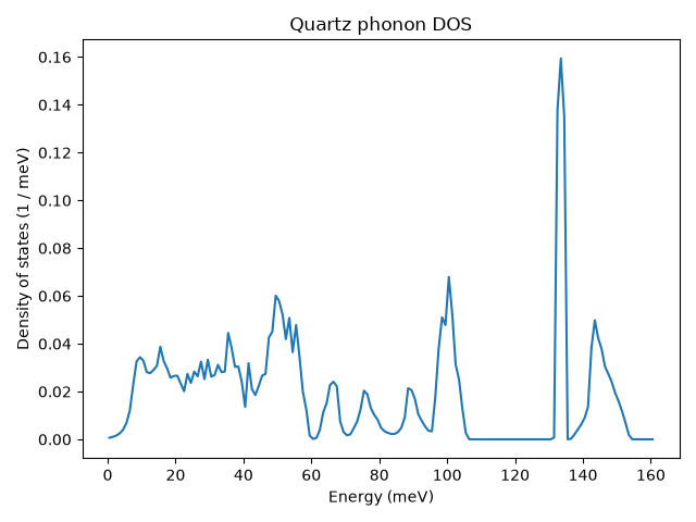
The output is a native AiiDA XyData (energy vs DOS).

import matplotlib.pyplot as plt

dos = results["dos"]
_, energy, energy_unit = dos.get_x()
((_, density, dos_unit),) = dos.get_y()

fig, ax = plt.subplots()
ax.plot(energy, density)
ax.set_xlabel(f"Energy ({energy_unit})")
ax.set_ylabel(f"Density of states ({dos_unit})")
ax.set_title("Quartz phonon DOS")
fig.tight_layout()

Provenance

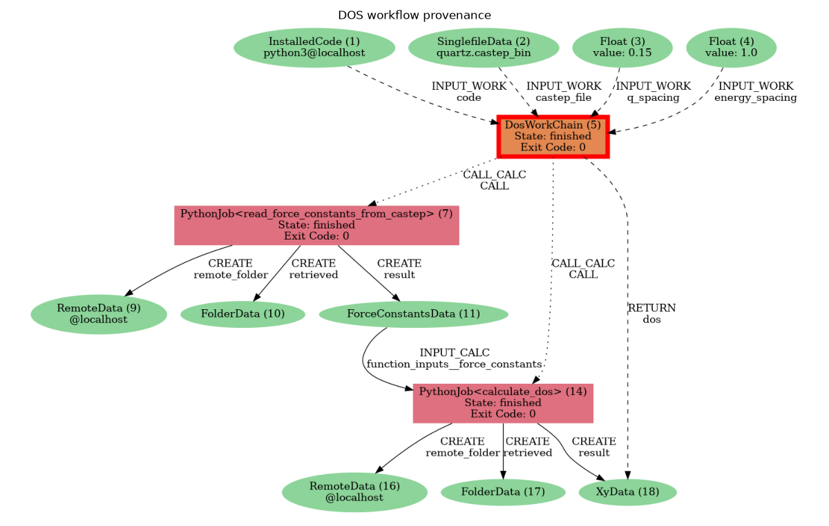
show_provenance(node, title="DOS workflow provenance")

<Figure size 1200x762.373 with 1 Axes>