TOSCA spectrum from precomputed phonon modes

Run ToscaFromModesWorkChain on ethanol phonon modes to simulate the inelastic-neutron-scattering spectrum the TOSCA spectrometer would record, plot it grouped two different ways, and visualise the AiiDA provenance graph.

Ethanol is a hydrogenous molecular crystal, which is what TOSCA is mostly used for: its almost-isotropic incoherent approximation is dominated by hydrogen, and published spectra for such samples are plentiful to compare against.

Set up AiiDA

A shared helper loads a temporary in-memory profile and a localhost Python code.

from _aiida_setup import example_data, get_python_code, show_provenance
from aiida import orm
from aiida.engine import run_get_node

code = get_python_code()

Load the phonon modes

The modes are a Euphonic QpointPhononModes JSON dump, which QpointPhononModesData reads directly – no conversion step is needed, because the node stores that JSON byte-for-byte.

from aiida.plugins import DataFactory, WorkflowFactory

# Load via the plugin factories (direct imports like
# `from aiida_pythonjob_ins.data import QpointPhononModesData` also work)
QpointPhononModesData = DataFactory("pythonjob_ins.qpoint_phonon_modes")
ToscaFromModesWorkChain = WorkflowFactory("pythonjob_ins.tosca_from_modes")

modes = QpointPhononModesData.from_json_file(
    example_data("ethanol_qpoint_phonon_modes.json")
)

Run the workflow, grouped by quantum order

The workflow computes the full, ungrouped line set as a PythonJob (one line per atom, quantum order and detector bank), then groups and broadens it. Both detector banks – backward at 135 degrees and forward at 45 degrees – are evaluated by default.

Caching is enabled explicitly rather than relying on the ambient configuration, so the second run below can demonstrably reuse the expensive step.

from aiida.manage.configuration import get_config

# The process type aiida-pythonjob registers PythonJob under.
PYTHONJOB_PROCESS_TYPE = "aiida.calculations:pythonjob.pythonjob"

# `aiida.manage.caching.enable_caching` is the usual way to do this in a script,
# but it is a context manager, and everything it covers would have to be indented
# into a single block -- which would collapse the separately explained steps below
# into one. Setting the option achieves the same thing without that constraint.
get_config().set_option("caching.enabled_for", [PYTHONJOB_PROCESS_TYPE])

by_order_results, by_order_node = run_get_node(
    ToscaFromModesWorkChain,
    modes=modes,
    temperature=orm.Float(10.0),  # kelvin
    energy_spacing=orm.Float(10.0),  # 1/cm
    group_by=orm.List(list=["quantum_order"]),
    code=code,
)
print(f"WorkChain finished OK: {by_order_node.is_finished_ok}")

WorkChain finished OK: True

Run again, grouped by element

Only the grouping keys differ, so the expensive intensity calculation is taken from the cache and only the cheap grouping and broadening steps run again. This is the point of committing the ungrouped line set to the graph as its own output.

by_element_results, by_element_node = run_get_node(
    ToscaFromModesWorkChain,
    modes=modes,
    temperature=orm.Float(10.0),
    energy_spacing=orm.Float(10.0),
    group_by=orm.List(list=["atom_symbol"]),
    code=code,
)
print(f"WorkChain finished OK: {by_element_node.is_finished_ok}")

WorkChain finished OK: True

Confirm the expensive step was reused rather than repeated. Asserting this means a silent loss of cacheability fails the documentation build instead of passing unnoticed.

intensity_jobs = [
    process
    for process in by_element_node.called_descendants
    if isinstance(process, orm.CalcJobNode)
]
reused = all(job.base.caching.is_created_from_cache for job in intensity_jobs)
print(f"Intensity calculation taken from the cache: {reused}")
assert reused, "expected the second run to reuse the cached intensity calculation"

Intensity calculation taken from the cache: True

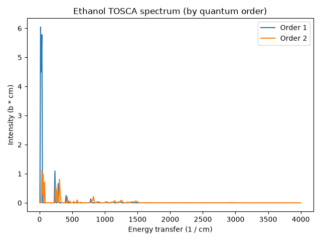
Plot the spectrum, grouped by quantum order

The output is a native AiiDA XyData: one x array of energies, one y array per group, each named with a ready-made legend label derived from the line’s metadata.

import matplotlib.pyplot as plt


def plot_spectrum(spectrum, title):
    """Plot every y array of an XyData spectrum, using its names as labels."""
    _, energy, energy_unit = spectrum.get_x()
    lines = spectrum.get_y()
    intensity_unit = lines[0][2]  # shared by every line of the collection

    fig, ax = plt.subplots()
    for label, intensity, _ in lines:
        ax.plot(energy, intensity, label=label)
    ax.set_xlabel(f"Energy transfer ({energy_unit})")
    ax.set_ylabel(f"Intensity ({intensity_unit})")
    ax.set_title(title)
    ax.legend()
    fig.tight_layout()
    return fig


plot_spectrum(by_order_results["spectrum"], "Ethanol TOSCA spectrum (by quantum order)")

<Figure size 640x480 with 1 Axes>

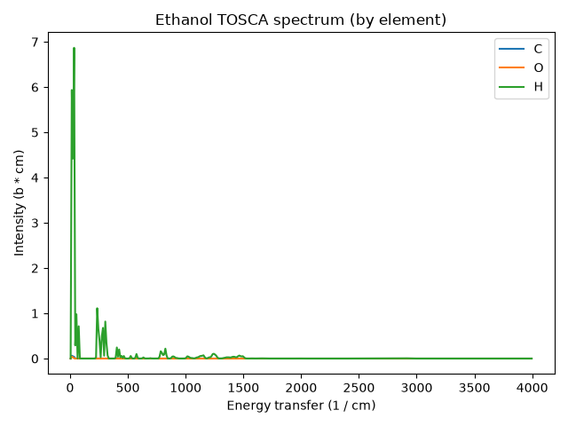
Plot the same calculation, grouped by element

Hydrogen dominates, as expected for an incoherent-approximation spectrum of a hydrogenous sample.

plot_spectrum(by_element_results["spectrum"], "Ethanol TOSCA spectrum (by element)")

<Figure size 640x480 with 1 Axes>

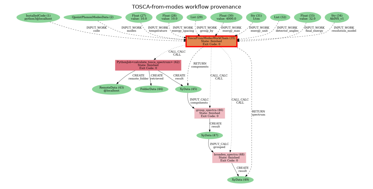
Provenance

The graph shows the single intensity PythonJob feeding the components output, and the grouping and broadening calcfunctions branching off it.

show_provenance(by_element_node, title="TOSCA-from-modes workflow provenance")

<Figure size 1200x608.473 with 1 Axes>