Molecular Dynamics

Set up environment (optional)

These steps are required to run this tutorial with Google Colab. To do so, uncomment and run the cell below.

This will replace pre-installed versions of numpy and torch in Colab with versions that are known to be compatible with janus-core.

It may be possible to skip the steps that uninstall and reinstall torch, which will save a considerable amount of time.

These instructions but may work for other systems too, but it is typically preferable to prepare a virtual environment separately before running this notebook if possible.

# import locale
# locale.getpreferredencoding = lambda: "UTF-8"

# ! pip uninstall numpy -y # Uninstall pre-installed numpy

# ! pip uninstall torch torchaudio torchvision transformers -y # Uninstall pre-installed torch
# ! uv pip install torch==2.5.1 # Install pinned version of torch

# ! uv pip install janus-core[mace,visualise] data-tutorials --system # Install janus-core with MACE and WeasWidget, and data-tutorials

# get_ipython().kernel.do_shutdown(restart=True) # Restart kernel to update libraries. This may warn that your session has crashed.

To ensure you have the latest version of janus-core installed, compare the output of the following cell to the latest version available at https://pypi.org/project/janus-core/

from janus_core import __version__

print(__version__)

0.8.3

Prepare data and modules

from ase.build import bulk
from weas_widget import WeasWidget
from ase.io import read
from data_tutorials.data import get_data
import matplotlib.pyplot as plt
import numpy as np

from janus_core.calculations.md import NVE, NVT
from janus_core.helpers.stats import Stats
from janus_core.processing import post_process

Use data_tutorials to get the data required for this tutorial:

get_data(
    url="https://raw.githubusercontent.com/stfc/janus-core/main/docs/source/tutorials/data/",
    filename=["precomputed_NaCl-traj.xyz"],
    folder="data",
)

try to download precomputed_NaCl-traj.xyz from https://raw.githubusercontent.com/stfc/janus-core/main/docs/source/tutorials/data/ and save it in data/precomputed_NaCl-traj.xyz

saved in data/precomputed_NaCl-traj.xyz

Cooling

Build NaCl structure and attach the MACE calculator:

NaCl = bulk("NaCl", "rocksalt", a=5.63, cubic=True)
NaCl = NaCl * (2, 2, 2)

v=WeasWidget()
v.from_ase(NaCl)
v

Prepare a simulation, cooling the structure from 300K to 200K in stepx of 20K, with 5fs at each temperature:

cooling = NVT(
    struct=NaCl.copy(),
    arch="mace_mp",
    device="cpu",
    model="small",
    calc_kwargs={"default_dtype": "float64"},
    temp_start=300.0,
    temp_end=200.0,
    temp_step=20,
    temp_time=5,
    stats_every=2,
)

/home/runner/work/janus-core/janus-core/.venv/lib/python3.12/site-packages/e3nn/o3/_wigner.py:10: UserWarning: Environment variable TORCH_FORCE_NO_WEIGHTS_ONLY_LOAD detected, since the`weights_only` argument was not explicitly passed to `torch.load`, forcing weights_only=False.
  _Jd, _W3j_flat, _W3j_indices = torch.load(os.path.join(os.path.dirname(__file__), 'constants.pt'))

cuequivariance or cuequivariance_torch is not available. Cuequivariance acceleration will be disabled.
Using Materials Project MACE for MACECalculator with /home/runner/.cache/mace/20231210mace128L0_energy_epoch249model
Using float64 for MACECalculator, which is slower but more accurate. Recommended for geometry optimization.
Using head Default out of ['Default']

/home/runner/work/janus-core/janus-core/.venv/lib/python3.12/site-packages/mace/calculators/mace.py:143: UserWarning: Environment variable TORCH_FORCE_NO_WEIGHTS_ONLY_LOAD detected, since the`weights_only` argument was not explicitly passed to `torch.load`, forcing weights_only=False.
  torch.load(f=model_path, map_location=device)

Run cooling:

cooling.run()

/home/runner/work/janus-core/janus-core/.venv/lib/python3.12/site-packages/ase/io/extxyz.py:318: UserWarning: Skipping unhashable information real_time
  warnings.warn('Skipping unhashable information '

All output files are saved in a results directory, janus_results.

Within this, the final structures at each temperature are saved in Cl32Na32-nvt-T300.0-final.xyz, Cl32Na32-nvt-T280.0-final.xyz, …, Cl32Na32-nvt-T200.0-final.xyz.

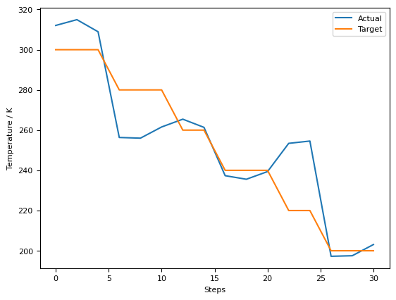
The statistics from the simulation are also saved every 20 steps in Cl32Na32-nvt-T300.0-T200.0-stats.dat. This can then be analysed using the Stats module:

data = Stats("janus_results/Cl32Na32-nvt-T300.0-T200.0-stats.dat")

print(data)

contains 17 timeseries, each with 16 elements
index label units
0 # Step
1 Real_Time s
2 Time fs
3 Epot/N eV
4 EKin/N eV
5 T K
6 ETot/N eV
7 Density g/cm^3
8 Volume Ang^3
9 P GPa
10 Pxx GPa
11 Pyy GPa
12 Pzz GPa
13 Pyz GPa
14 Pxz GPa
15 Pxy GPa
16 Target_T K

plt.plot(data[0], data[5], label="Actual")
plt.plot(data[0], data[16], label="Target")
plt.legend()
plt.xlabel("Steps")
plt.ylabel("Temperature / K")
plt.show()

Heating, followed by MD

This will prepare an NVT MD simulation, initially increasing the temperature from 0K to 300K in 20K steps, with 1fs at each temperature, before a further 10 steps (10fs) at 300K.

The final structure at each temperature will be saved, e.g. Cl32Na32-nvt-T0-final.xyz, Cl32Na32-nvt-T0-final.xyz, …, Cl32Na32-nvt-T300-final.xyz.

heating = NVT(
    struct=NaCl.copy(),
    arch="mace_mp",
    device="cpu",
    model="small",
    calc_kwargs={"default_dtype": "float64"},
    temp_start=0,  # Start of temperature ramp
    temp_end=300.0,  # End of temperature ramp
    temp_step=20,  # Temperature ramp increments
    temp_time=1,  # Time at each temperature in ramp
    temp=300,  # MD temperature
    steps=10,  # MD steps at 300K
)

Using Materials Project MACE for MACECalculator with /home/runner/.cache/mace/20231210mace128L0_energy_epoch249model
Using float64 for MACECalculator, which is slower but more accurate. Recommended for geometry optimization.
Using head Default out of ['Default']

/home/runner/work/janus-core/janus-core/.venv/lib/python3.12/site-packages/mace/calculators/mace.py:143: UserWarning: Environment variable TORCH_FORCE_NO_WEIGHTS_ONLY_LOAD detected, since the`weights_only` argument was not explicitly passed to `torch.load`, forcing weights_only=False.
  torch.load(f=model_path, map_location=device)

heating.run()

/home/runner/work/janus-core/janus-core/.venv/lib/python3.12/site-packages/ase/io/extxyz.py:318: UserWarning: Skipping unhashable information real_time
  warnings.warn('Skipping unhashable information '

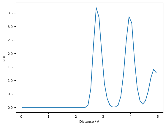
The same structure can then be used to run an additional NVE MD simulation for 50 steps (50fs), with post-processing performed to compute the RDF by setting post_process_kwargs = {"rdf_compute": True}, with the results saved to Cl32Na32-nve-rdf.dat:

md = NVE(
    struct=heating.struct,
    temp=300,
    stats_every=5,
    steps=50,
    post_process_kwargs={"rdf_compute": True, "rdf_rmax": 5, "rdf_bins": 50},
)

md.run()

# view trajectory

v=WeasWidget()
traj = read("data/precomputed_NaCl-traj.xyz", index=":")
v.from_ase(traj)
v.avr.model_style = 1
v.avr.show_hydrogen_bonds = True
v

rdf = np.loadtxt("janus_results/Cl32Na32-nve-T300-rdf.dat")
bins, counts = zip(*rdf)

plt.plot(bins, counts)
plt.ylabel("RDF")
plt.xlabel("Distance / Å")
plt.show()

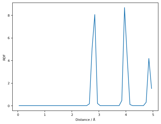
The same post-processing can also be performed separately after completing the simulation:

data = read("data/precomputed_NaCl-traj.xyz", index=":")

rdf = post_process.compute_rdf(traj, rmax=5.0, nbins=50)

plt.plot(rdf[0], rdf[1])
plt.ylabel("RDF")
plt.xlabel("Distance / Å")
plt.show()