![]()
Nudged Elastic Band
In this tutorial, we will determine the activation energies of Li diffusion along the [010] and [001] directions (referred to as paths b and c respectively) in lithium iron phosphate (LiFePO_4), a cathode material for lithium ion batteries.
DFT references energies are:
Barrier heights:
path b = 0.27 eV
path c = 2.5 eV
(see table 1 in https://doi.org/10.1039/C5TA05062F)
Set up environment (optional)
These steps are required to run this tutorial with Google Colab. To do so, uncomment and run the cell below.
This will replace pre-installed versions of numpy and torch in Colab with versions that are known to be compatible with janus-core.
It may be possible to skip the steps that uninstall and reinstall torch, which will save a considerable amount of time.
These instructions but may work for other systems too, but it is typically preferable to prepare a virtual environment separately before running this notebook if possible.
[1]:
# import locale
# locale.getpreferredencoding = lambda: "UTF-8"
# ! pip uninstall numpy -y # Uninstall pre-installed numpy
# ! pip uninstall torch torchaudio torchvision transformers -y # Uninstall pre-installed torch
# ! uv pip install torch==2.5.1 # Install pinned version of torch
# ! uv pip install janus-core[mace,orb,chgnet,visualise] data-tutorials --system # Install janus-core with MACE, Orb, CHGNet, and WeasWidget, and data-tutorials
# get_ipython().kernel.do_shutdown(restart=True) # Restart kernel to update libraries. This may warn that your session has crashed.
To ensure you have the latest version of janus-core installed, compare the output of the following cell to the latest version available at https://pypi.org/project/janus-core/
[2]:
from janus_core import __version__
print(__version__)
0.9.3
Prepare data, modules, and model parameters
You can toggle the following to investigate different models:
[3]:
model_params = {"arch": "mace_mp", "model": "medium-0b3"}
# model_params = {"arch": "mace_mp", "model": "medium-mpa-0"}
# model_params = {"arch": "mace_mp", "model": "medium-omat-0"}
# model_params = {"arch": "chgnet"}
# model_params = {"arch": "orb"}
[4]:
from weas_widget import WeasWidget
from ase.io import read
from data_tutorials.data import get_data
from janus_core.calculations.geom_opt import GeomOpt
from janus_core.calculations.neb import NEB
Use data_tutorials to get the data required for this tutorial:
[5]:
get_data(
url="https://raw.githubusercontent.com/stfc/janus-core/main/docs/source/tutorials/data/",
filename="LiFePO4_supercell.cif",
folder="data",
)
try to download LiFePO4_supercell.cif from https://raw.githubusercontent.com/stfc/janus-core/main/docs/source/tutorials/data/ and save it in data/LiFePO4_supercell.cif
saved in data/LiFePO4_supercell.cif
Preparing end structures
The initial structure can be downloaded from the Materials Project (mp-19017):
[6]:
LFPO = read("data/LiFePO4_supercell.cif")
v=WeasWidget()
v.from_ase(LFPO)
v.avr.model_style = 1
v.avr.show_hydrogen_bonds = True
v
[6]:
First, we will relax the supercell:
[7]:
GeomOpt(struct=LFPO, **model_params).run()
v1=WeasWidget()
v1.from_ase(LFPO)
v1.avr.model_style = 1
v1.avr.show_hydrogen_bonds = True
v1
/home/runner/work/janus-core/janus-core/.venv/lib/python3.12/site-packages/e3nn/o3/_wigner.py:10: UserWarning: Environment variable TORCH_FORCE_NO_WEIGHTS_ONLY_LOAD detected, since the`weights_only` argument was not explicitly passed to `torch.load`, forcing weights_only=False.
_Jd, _W3j_flat, _W3j_indices = torch.load(os.path.join(os.path.dirname(__file__), 'constants.pt'))
cuequivariance or cuequivariance_torch is not available. Cuequivariance acceleration will be disabled.
Downloading MACE model from 'https://github.com/ACEsuit/mace-mp/releases/download/mace_mp_0b3/mace-mp-0b3-medium.model'
Cached MACE model to /home/runner/.cache/mace/macemp0b3mediummodel
Using Materials Project MACE for MACECalculator with /home/runner/.cache/mace/macemp0b3mediummodel
Using float64 for MACECalculator, which is slower but more accurate. Recommended for geometry optimization.
/home/runner/work/janus-core/janus-core/.venv/lib/python3.12/site-packages/mace/calculators/mace.py:199: UserWarning: Environment variable TORCH_FORCE_NO_WEIGHTS_ONLY_LOAD detected, since the`weights_only` argument was not explicitly passed to `torch.load`, forcing weights_only=False.
torch.load(f=model_path, map_location=device)
Step Time Energy fmax
LBFGS: 0 10:59:54 -762.842666 0.654854
LBFGS: 1 10:59:56 -763.038742 0.437508
LBFGS: 2 10:59:58 -763.090096 0.392867
LBFGS: 3 11:00:00 -763.119488 0.374220
LBFGS: 4 11:00:02 -763.172830 0.346620
LBFGS: 5 11:00:04 -763.213488 0.334927
LBFGS: 6 11:00:06 -763.256842 0.327520
LBFGS: 7 11:00:08 -763.297792 0.328964
LBFGS: 8 11:00:09 -763.342419 0.332009
LBFGS: 9 11:00:11 -763.385108 0.328513
LBFGS: 10 11:00:13 -763.427187 0.308144
LBFGS: 11 11:00:15 -763.474267 0.274918
LBFGS: 12 11:00:17 -763.528185 0.234548
LBFGS: 13 11:00:18 -763.579927 0.246328
LBFGS: 14 11:00:20 -763.627605 0.245408
LBFGS: 15 11:00:22 -763.684752 0.231582
LBFGS: 16 11:00:24 -763.766360 0.283626
LBFGS: 17 11:00:25 -763.855346 0.296599
LBFGS: 18 11:00:27 -763.931149 0.188692
LBFGS: 19 11:00:29 -763.965778 0.154808
LBFGS: 20 11:00:31 -763.996599 0.213159
LBFGS: 21 11:00:32 -764.039520 0.255107
LBFGS: 22 11:00:34 -764.108589 0.255570
LBFGS: 23 11:00:36 -764.175608 0.200210
LBFGS: 24 11:00:38 -764.208816 0.096659
[7]:
Next, we will create the start and end structures:
[8]:
# NEB path along b and c directions have the same starting image.
# For start bc remove site 5
LFPO_start_bc = LFPO.copy()
del LFPO_start_bc[5]
# For end b remove site 11
LFPO_end_b = LFPO.copy()
del LFPO_end_b[11]
# For end c remove site 4
LFPO_end_c = LFPO.copy()
del LFPO_end_c[4]
Path b
We can now calculate the barrier height along path b.
This also includes running geometry optimization on the end points of this path.
[9]:
n_images = 7
interpolator="pymatgen" # ASE interpolation performs poorly in this case
neb_b = NEB(
init_struct=LFPO_start_bc,
final_struct=LFPO_end_b,
n_images=n_images,
interpolator=interpolator,
minimize=True,
fmax=0.1,
**model_params,
)
Using Materials Project MACE for MACECalculator with /home/runner/.cache/mace/macemp0b3mediummodel
Using float64 for MACECalculator, which is slower but more accurate. Recommended for geometry optimization.
/home/runner/work/janus-core/janus-core/.venv/lib/python3.12/site-packages/mace/calculators/mace.py:199: UserWarning: Environment variable TORCH_FORCE_NO_WEIGHTS_ONLY_LOAD detected, since the`weights_only` argument was not explicitly passed to `torch.load`, forcing weights_only=False.
torch.load(f=model_path, map_location=device)
[10]:
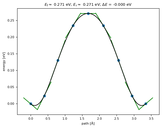
results = neb_b.run()
Step Time Energy fmax
LBFGS: 0 11:00:39 -758.975432 1.930990
LBFGS: 1 11:00:41 -759.140669 0.711957
LBFGS: 2 11:00:43 -759.209571 0.514600
LBFGS: 3 11:00:45 -759.298948 0.404890
LBFGS: 4 11:00:46 -759.316304 0.265548
LBFGS: 5 11:00:48 -759.336518 0.252446
LBFGS: 6 11:00:50 -759.351338 0.330410
LBFGS: 7 11:00:51 -759.368546 0.309163
LBFGS: 8 11:00:53 -759.378014 0.229741
LBFGS: 9 11:00:55 -759.386280 0.221552
LBFGS: 10 11:00:56 -759.395290 0.278156
LBFGS: 11 11:00:58 -759.404981 0.291370
LBFGS: 12 11:01:00 -759.411852 0.192426
LBFGS: 13 11:01:01 -759.415355 0.075502
Step Time Energy fmax
LBFGS: 0 11:01:03 -758.975436 1.930961
LBFGS: 1 11:01:05 -759.140671 0.711930
LBFGS: 2 11:01:07 -759.209572 0.514582
LBFGS: 3 11:01:08 -759.298949 0.404887
LBFGS: 4 11:01:10 -759.316305 0.265544
LBFGS: 5 11:01:12 -759.336519 0.252446
LBFGS: 6 11:01:13 -759.351338 0.330395
LBFGS: 7 11:01:15 -759.368546 0.309158
LBFGS: 8 11:01:17 -759.378015 0.229745
LBFGS: 9 11:01:19 -759.386281 0.221556
LBFGS: 10 11:01:20 -759.395291 0.278147
LBFGS: 11 11:01:22 -759.404982 0.291359
LBFGS: 12 11:01:24 -759.411852 0.192423
LBFGS: 13 11:01:25 -759.415355 0.075502
/home/runner/work/janus-core/janus-core/.venv/lib/python3.12/site-packages/ase/mep/neb.py:329: UserWarning: The default method has changed from 'aseneb' to 'improvedtangent'. The 'aseneb' method is an unpublished, custom implementation that is not recommended as it frequently results in very poor bands. Please explicitly set method='improvedtangent' to silence this warning, or set method='aseneb' if you strictly require the old behavior (results may vary). See: https://gitlab.com/ase/ase/-/merge_requests/3952
warnings.warn(
Step Time fmax
NEBOptimizer[ode]: 0 11:02:04 1.5090
NEBOptimizer[ode]: 1 11:02:16 1.1032
NEBOptimizer[ode]: 2 11:02:28 0.9983
NEBOptimizer[ode]: 3 11:02:40 0.8704
NEBOptimizer[ode]: 4 11:02:52 0.8013
NEBOptimizer[ode]: 5 11:03:03 0.7712
NEBOptimizer[ode]: 6 11:03:15 0.7441
NEBOptimizer[ode]: 7 11:03:27 0.6738
NEBOptimizer[ode]: 8 11:03:39 0.4347
NEBOptimizer[ode]: 9 11:04:02 0.4299
NEBOptimizer[ode]: 10 11:04:14 0.4227
NEBOptimizer[ode]: 11 11:04:26 0.3947
NEBOptimizer[ode]: 12 11:04:37 0.2843
NEBOptimizer[ode]: 13 11:05:01 0.2726
NEBOptimizer[ode]: 14 11:05:13 0.2653
NEBOptimizer[ode]: 15 11:05:24 0.2612
NEBOptimizer[ode]: 16 11:05:36 0.2552
NEBOptimizer[ode]: 17 11:05:48 0.2323
NEBOptimizer[ode]: 18 11:06:12 0.2219
NEBOptimizer[ode]: 19 11:06:24 0.2141
NEBOptimizer[ode]: 20 11:06:36 0.2087
NEBOptimizer[ode]: 21 11:06:48 0.2056
NEBOptimizer[ode]: 22 11:06:59 0.2005
NEBOptimizer[ode]: 23 11:07:11 0.1808
NEBOptimizer[ode]: 24 11:07:35 0.1730
NEBOptimizer[ode]: 25 11:07:47 0.1667
NEBOptimizer[ode]: 26 11:07:59 0.1626
NEBOptimizer[ode]: 27 11:08:10 0.1600
NEBOptimizer[ode]: 28 11:08:22 0.1561
NEBOptimizer[ode]: 29 11:08:34 0.1408
NEBOptimizer[ode]: 30 11:08:58 0.1351
NEBOptimizer[ode]: 31 11:09:09 0.1303
NEBOptimizer[ode]: 32 11:09:21 0.1271
NEBOptimizer[ode]: 33 11:09:33 0.1249
NEBOptimizer[ode]: 34 11:09:45 0.1217
NEBOptimizer[ode]: 35 11:09:56 0.1092
NEBOptimizer[ode]: 36 11:10:20 0.1058
NEBOptimizer[ode]: 37 11:10:32 0.1033
NEBOptimizer[ode]: 38 11:10:43 0.1008
NEBOptimizer[ode]: 39 11:10:55 0.0974
The results include the barrier (without any interpolation between highest images) and maximum force at the point in the simulation
[11]:
print(results)
{'barrier': np.float64(0.2871329749605138), 'delta_E': np.float64(-1.6499575394846033e-07), 'max_force': np.float64(0.10735346812660264)}
We can also plot the band:
[12]:
fig = neb_b.nebtools.plot_band()
v1=WeasWidget()
v1.from_ase(neb_b.nebtools.images)
v1.avr.model_style = 1
v1.avr.show_hydrogen_bonds = True
v1
[12]:
Path c
We can calculate the barrier height along path c similarly
[13]:
n_images = 7
interpolator="pymatgen"
neb_c = NEB(
init_struct=LFPO_start_bc,
final_struct=LFPO_end_c,
n_images=n_images,
interpolator=interpolator,
minimize=True,
fmax=0.1,
**model_params,
)
Using Materials Project MACE for MACECalculator with /home/runner/.cache/mace/macemp0b3mediummodel
Using float64 for MACECalculator, which is slower but more accurate. Recommended for geometry optimization.
/home/runner/work/janus-core/janus-core/.venv/lib/python3.12/site-packages/mace/calculators/mace.py:199: UserWarning: Environment variable TORCH_FORCE_NO_WEIGHTS_ONLY_LOAD detected, since the`weights_only` argument was not explicitly passed to `torch.load`, forcing weights_only=False.
torch.load(f=model_path, map_location=device)
[14]:
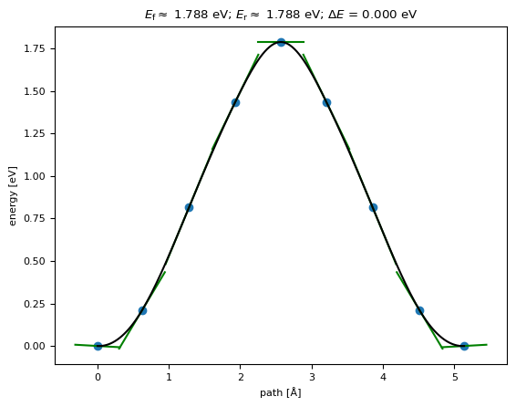
results = neb_c.run()
Step Time Energy fmax
LBFGS: 0 11:11:13 -759.415355 0.075502
Step Time Energy fmax
LBFGS: 0 11:11:14 -758.975431 1.930990
LBFGS: 1 11:11:16 -759.140669 0.711958
LBFGS: 2 11:11:18 -759.209571 0.514601
LBFGS: 3 11:11:19 -759.298948 0.404890
LBFGS: 4 11:11:21 -759.316304 0.265548
LBFGS: 5 11:11:23 -759.336518 0.252446
LBFGS: 6 11:11:25 -759.351338 0.330410
LBFGS: 7 11:11:26 -759.368546 0.309163
LBFGS: 8 11:11:28 -759.378014 0.229741
LBFGS: 9 11:11:30 -759.386280 0.221553
LBFGS: 10 11:11:31 -759.395290 0.278156
LBFGS: 11 11:11:33 -759.404981 0.291370
LBFGS: 12 11:11:35 -759.411852 0.192426
LBFGS: 13 11:11:36 -759.415355 0.075502
/home/runner/work/janus-core/janus-core/.venv/lib/python3.12/site-packages/ase/mep/neb.py:329: UserWarning: The default method has changed from 'aseneb' to 'improvedtangent'. The 'aseneb' method is an unpublished, custom implementation that is not recommended as it frequently results in very poor bands. Please explicitly set method='improvedtangent' to silence this warning, or set method='aseneb' if you strictly require the old behavior (results may vary). See: https://gitlab.com/ase/ase/-/merge_requests/3952
warnings.warn(
Step Time fmax
NEBOptimizer[ode]: 0 11:12:15 2.3205
NEBOptimizer[ode]: 1 11:12:27 1.6499
NEBOptimizer[ode]: 2 11:12:39 0.9977
NEBOptimizer[ode]: 3 11:12:51 0.6537
NEBOptimizer[ode]: 4 11:13:14 0.4186
NEBOptimizer[ode]: 5 11:13:26 0.3969
NEBOptimizer[ode]: 6 11:13:38 0.3176
NEBOptimizer[ode]: 7 11:14:01 0.2998
NEBOptimizer[ode]: 8 11:14:25 0.2691
NEBOptimizer[ode]: 9 11:14:37 0.2608
NEBOptimizer[ode]: 10 11:14:49 0.2293
NEBOptimizer[ode]: 11 11:15:12 0.2186
NEBOptimizer[ode]: 12 11:15:24 0.2605
NEBOptimizer[ode]: 13 11:15:36 0.2010
NEBOptimizer[ode]: 14 11:15:47 0.1946
NEBOptimizer[ode]: 15 11:15:59 0.1884
NEBOptimizer[ode]: 16 11:16:11 0.1653
NEBOptimizer[ode]: 17 11:16:35 0.1601
NEBOptimizer[ode]: 18 11:16:47 0.1541
NEBOptimizer[ode]: 19 11:16:59 0.1474
NEBOptimizer[ode]: 20 11:17:10 0.1470
NEBOptimizer[ode]: 21 11:17:22 0.1335
NEBOptimizer[ode]: 22 11:17:34 0.1272
NEBOptimizer[ode]: 23 11:17:46 0.1249
NEBOptimizer[ode]: 24 11:17:58 0.1146
NEBOptimizer[ode]: 25 11:18:10 0.1210
NEBOptimizer[ode]: 26 11:18:33 0.1307
NEBOptimizer[ode]: 27 11:18:45 0.0743
[15]:
print(results)
{'barrier': np.float64(1.783796087908737), 'delta_E': np.float64(4.249386620358564e-09), 'max_force': np.float64(0.08880301852155578)}
[16]:
fig = neb_c.nebtools.plot_band()
v2=WeasWidget()
v2.from_ase(neb_c.nebtools.images)
v2.avr.model_style = 1
v2.avr.show_hydrogen_bonds = True
v2
[16]:
Continuing NEBs
You can also continue a NEB to a tighter fmax:
[17]:
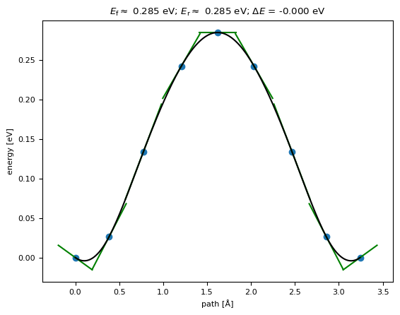
neb_b.optimize(fmax=0.05)
neb_b.run_nebtools()
print(neb_b.results)
fig = neb_b.nebtools.plot_band()
v1=WeasWidget()
v1.from_ase(neb_b.nebtools.images)
v1.avr.model_style = 1
v1.avr.show_hydrogen_bonds = True
v1
NEBOptimizer[ode]: 40 11:19:24 0.1017
NEBOptimizer[ode]: 41 11:19:47 0.0727
NEBOptimizer[ode]: 42 11:19:59 0.0716
NEBOptimizer[ode]: 43 11:20:11 0.0674
NEBOptimizer[ode]: 44 11:20:23 0.0514
NEBOptimizer[ode]: 45 11:20:35 0.0375
{'barrier': np.float64(0.2708174321553542), 'delta_E': np.float64(-1.6499575394846033e-07), 'max_force': np.float64(0.039658769622492145)}
[17]:
It is also possible to change NEB parameters, accessed through the attributes of NEB.neb, such as to continue or retry a NEB using different methods.
Note that although the “success” of the NEB optimisation can be accessed through NEB.converged, this is typically only set to False if a OptimizerConvergenceError, not when the maximum number of steps is reached. We therefore recommend checking NEB.opt.nsteps or NEB.results["max_force"].
[18]:
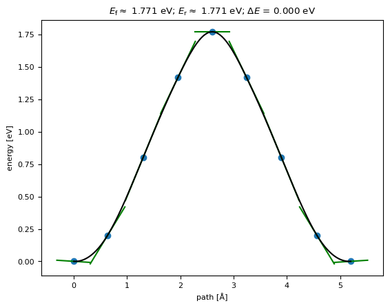
neb_c.neb.climb = True
neb_c.run(fmax=0.05)
print(neb_c.results)
print(neb_c.opt.nsteps)
fig = neb_c.nebtools.plot_band()
v1=WeasWidget()
v1.from_ase(neb_c.nebtools.images)
v1.avr.model_style = 1
v1.avr.show_hydrogen_bonds = True
v1
NEBOptimizer[ode]: 28 11:21:10 0.1167
NEBOptimizer[ode]: 29 11:21:34 0.1040
NEBOptimizer[ode]: 30 11:21:46 0.0432
{'barrier': np.float64(1.7708297606136476), 'delta_E': np.float64(4.249386620358564e-09), 'max_force': np.float64(0.05601022200402612)}
31
[18]: